2 Bayes’ theorem
Alright! Earlier we covered Bayesian statistics and a bit of probability - now let’s get into the most important theorem of all!
The almighty Bayes’ theorem!
Bayes’ theorem is literally the backbone of this field (no points for guessing where the name Bayesian Statistics comes from).
Bayes theorem is based on conditional probability.
i.e. finding the probability of event A happening, given we know event B already happened.
Let’s first see an example to understand conditional probability!
2.1 Challenge 1: Sorting the Staff
Q) There are 20 employees at a company, 12 of whom are female. There are 10 PhDs, of which 6 are female. What is the probability of being a female given they have a PhD?
You can solve this mentally too but let’s try to solve this using a simple table.
Based on the data given to us we can create the below table:
Our job is to find the missing data values. As you can see this is fairly easy to solve -
Based on the data given to us we can create the following table:
| Female | Male | Total | |
|---|---|---|---|
| PhDs | 6 | ? | 10 |
| Not PhDs | ? | ? | ? |
| Total | 12 | ? | 20 |
Our job is to find the missing data values. As you can see this is fairly easy to solve
| Female | Male | Total | |
|---|---|---|---|
| PhDs | 6 | 4 | 10 |
| Not PhDs | 6 | 4 | 10 |
| Total | 12 | 8 | 20 |
We are asked what is P(F|PhD)?
The total number of PhDs = 10. Of which the number of females = 6.
Thus, the universe size is 10 and we want to find the probability of being female.
That equates to, P(F|PhD) = 6/10
We can arrive at the same conclusion in a different way using conditional probabilities which is given as,
\(P(A|B) = \frac{P(A ∩ B)}{P(B)}\)
Substituting the above equation with our example we get,
\(P(F|PhD) = \frac{P(F ∩ PhD)}{P(PhD)}\)
Translating the above equation in English you will see it matches our earlier statement:
From the universe of PhDs (denominator) we want to find all those that are female AND have a PhD (numerator).
Let’s find each of the elements in this equation:
First, let’s get the probability of being a female on this team. This is known as marginal probability.
For P(F) we find total number of females and divide by total count.
P(F) = \(\frac{12}{20} = \frac{3}{5}\) … marginal probability
Similarly, the probability of having a PhD is,
P(PhD) = \(\frac{10}{20} = \frac{1}{2}\) … marginal probability
Next, to find the probability of being female and having a PhD,
find the cell that corresponds to female and PhD (= 6), divide this with the total number (=20). This is known as the joint probability.
P(F ∩ PhD) = \(\frac{6}{20} = \frac{3}{10}\) … joint probability
Now that we have all these elements in place we can find P(F | PhD). This is known as conditional probability and is given by,
P(F|PhD) \(= \frac{P(F ∩ PhD)}{P(PhD)}\)
P(F|PhD) \(= \frac{3/10}{1/2} = \frac{6}{10}\) … conditional probability
This matches the answer we had seen earlier. This was just a different way to get to it.
2.2 Deriving the Bayes Theorem
Okay, now that we have seen that example let’s look at some equations and derive the Bayes theorem
In mathematical form, the conditional probability is given as:
\(P(A|B) = \frac{P(A \cap B)}{P(B)}\) … eqn(1)
i.e. The probability of A given B is the probability that A and B happen together relative to the probability that B happens at all.
Lets look at equation 1 again -
\(P(A|B) = \frac{P(A \cap B)}{P(B)}\)
Therefore, \(P(A|B) * P(B) = P(A \cap B)\)
Similarly, we can do the same manipulation for P(B|A) to get
\(P(B|A) * P(A) = P(A \cap B)\)
Since both the RHS values on the above equations are the same we know these equations are equal.
Therefore,
\(P(A|B) * P(B) = P(B|A) * P(A)\)
\[P(A|B) = \frac{P(B|A) * P(A)}{P(B)}\]
This is the Bayes theorem!
Why is this so great? Because if we are given the conditional probability of one event, we can use the theorem to find the conditional probability in the opposite direction.
I.e. if we know P(B|A) we can find P(A|B)
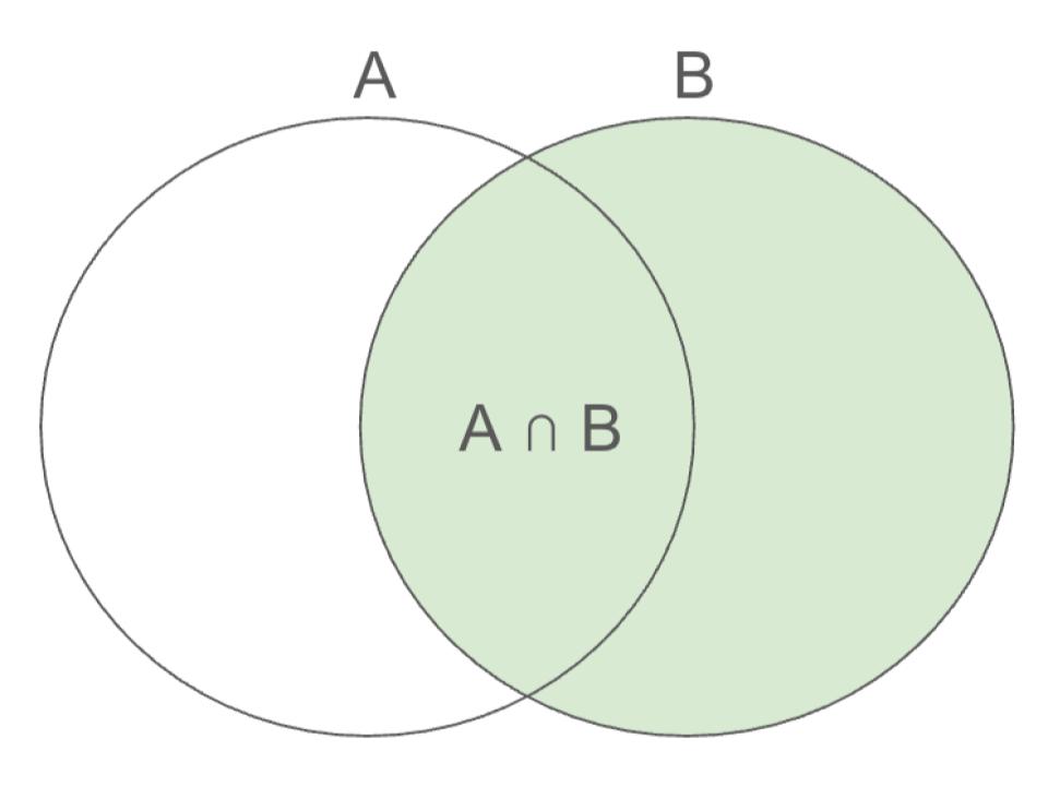
The numerator of the Bayes’ rule is the joint probability P(A ∩ B), and the denominator is the marginal probability P(B)
2.4 Challenge 2: Positive Result, Uncertain Reality: Decoding Cancer Probability
Yudkowsky in his Bayes article has given a great example - let’s have a look
Q) 1% of women at age forty who participate in routine screening have breast cancer. 80% of women with breast cancer will get positive mammographies. 9.6% of women without breast cancer will also get positive mammographies. A woman in this age group had a positive mammography in a routine screening. What is the probability that she actually has breast cancer?
Let’s write this down -
P(BC) = 1% = 0.01 therefore, P(~BC) = 99% = 0.99
P(+ | BC) = 80%
P(+ | ~BC) = 9.6%
P(BC | +) = ?
We will solve this using the equations we saw previously and also see it in table format
With Equations
Using Bayes theorem,
\(P(BC|+) = \frac{P(+|BC) * P(BC)}{P(+)}\)
We already have the values of the numerator. The objective then becomes to find the denominator and we are done!
What is the probability of testing positive?
\(P(+) = P(+ \cap BC) + P(+ \cap \bar{BC})\) …remember the venn diagram earlier?
\(P(+ \cap BC) = P(+|BC) * P(BC) = 0.8 * 0.01 = 0.008\)
\(P(+ \cap \bar{BC}) = P(+| \bar{BC}) * P( \bar{BC}) = 0.096 * 0.99 = 0.0905\)
Therefore,
\(P(+) = 0.008+0.0905 = 0.10304\)
Plugging this value back in to the bayes theorem we get -
\(P(BC|+) = \frac{0.8 * 0.01}{0.10304} = 7.7\%\)
Turns out, even if you test positive, there’s only a 7.7% chance you actually have cancer! Crazy, right?!
Isn’t that so counterintuitive!? We just saw that when you truly have breast cancer, the test gives a positive result 80% of the time but when we reverse the probability, we see that if we test positive on a test, the probability of you actually having cancer is just 7.7% !!
Not convinced? Let’s look at this using tables
Using Tables
From the question we know \(P(BC) = 1% = 0.01\); \(P(\bar{BC}) = 99% = 0.99\)
\(P(+ | BC) = 0.8\)
Using these two values we can find \(P(+ \cap BC)\)
\(P(+ \cap BC) = P(+|BC) * P(BC) = 0.8*0.01 = 0.008\)
From the question we also know P(+|~BC) = 9.6% = 0.096
\(P(+ \cap \bar{BC}) = P(+| \bar{BC}) * P(\bar{BC}) = 0.096*0.99 = 0.095\)
Let’s put these values in a table
| Cancer | No Cancer | Total | |
|---|---|---|---|
| Positive | 0.008 | 0.095 | 0.103 |
| Negative | 0.002 | 0.895 | 0.897 |
| Total | 0.01 | 0.99 | 1 |
Using Bayes theorem,
\(P(BC|+) = \frac{P(+|BC) * P(BC)}{P(+)}\)
\(P(BC|+) = \frac{(0.008 /0.01) * 0.01}{0.10304} = 7.7\%\)
We were given the probability of a positive result given a cancer condition and using Bayes theorem we were able to find the probability of cancer given we had a positive result.
2.5 Mission Complete: Summary
In this chapter we saw the almighty Bayes theorem and derived it too.
Remember, whenever you are given the probability of one direction and are asked the probability of the other direction you can use the Bayes theorem.
Alright! Let’s recap the main equations we need to be aware of
\[P(A|B) = \frac{P(A ∩ B)}{P(B)}\] \[P(A|B) = \frac{P(B|A) * P(A)}{P(B)}\] \[P(A|B) = \frac{P(B|A) * P(A)}{P(B \cap A) + P(B \cap \bar{A})}\] \[P(A|B) = \frac{P(B|A) * P(A)}{P(B | A) * P(A) + P(B | \bar{A}) * P(\bar{A})}\]
These are multiple ways of writing the same equation!
2.6 Skill Tree Extensions: Recommended Readings
- Yudkowsky’s Bayes article [HIGHLY RECOMMEND!!!]
- Bayesian Statistics the Fun Way book (Will Kurt)
- Will Kurt’s blog (countbayesie.com) - Bayes
- Bayesian Statistics for Beginners book (Donovan and Mickey)
- Doing Bayesian Data Analysis book (John Kruschke)
- Bayesian Statistics: From Concept to Data Analysis (Coursera)