Up until this point we have used shortcuts to compute posterior distributions. This worked fine for our datasets where there was a conjugate prior perfectly present for our likelihood function. But what if we have a likelihood function for which there is no conjugate prior? Or what if we have a likelihood function with an unknown conjugate prior? This is more common in the real world. In such cases, we need to use a different approach to compute the posterior distribution without having to do the integration in Bayes theorem. This is where Markov Chain Monte Carlo (MCMC) Simulations come in.
MCMC simulations are an approximation tool that allow us to compute posterior distributions without having to do the integration in Bayes theorem.
We had earlier seen that in the absence of the denominator, the Bayes theorem can be written as: \[\text{Posterior} \propto \text{Prior} \times \text{Likelihood}\]
Using MCMC we can approximate the posterior by taking multiple values of the prior and likelihood and combining them together to get a distribution that closely matches the actual posterior.
We can use MCMC simulations for all sorts of computations and later on in this section we will see how it can be used to run a regression and solve other inference problems.
Monte Carlo Simulations
Monte Carlo simulation is a simulation technique that uses random sampling to model systems involving uncertainty. It builds a model of possible results by using a probability distribution for any variable that has some uncertainty.
It’s like playing a game of ‘what if’ many times. It’s a beautiful concept because in essence it allows you to play god and see how a situation would look if it played out thousands and thousands of times.
How does it work?
Identify the uncertainty: There are things we don’t know for sure but yet we need to estimate. These are your uncertainties
Define the possibilities: for every uncertainty, you define a range of possible values it could take. Ie. define the distribution
Run ‘what if’ scenarios: the simulation randomly picks a value for each uncertainty based on the range you defined. It does this over and over again
Record the outcome: Each time a simulation runs, a ‘what if’ outcome gets calculated based on the random values picked
Analyze the results: After running all the scenarios, you end up with a huge collection of possible outcomes. You can now see the full range of possibilities.
Lucky number 10
Let’s see the Monte Carlo simulation in action with a very simple example:
Let there be two six-sided dice being rolled. You want to find the probability of getting a sum of at least 10.
How would you run this using the Monte Carlo simulation?
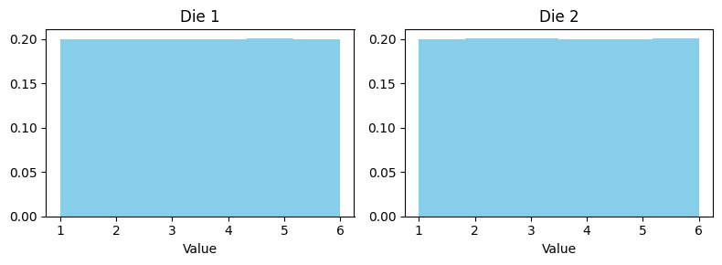
Step 1: every face of the die can show up equally, therefore this can be modeled as a uniform distribution with range 1 through 6
Step 2: set the simulation to run 1M times (because why not)
Step 3: for each run, find the sum of the values from the dice
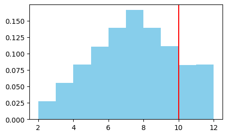
Step 4: Plot the output and see the distribution
Step 5: Find % of rolls that are greater than 10
Code
# code-fold: false import numpy as npimport pandas as pdimport matplotlib.pyplot as pltsims =1000000num1 = np.random.randint(1,7, sims)num2 = np.random.randint(1,7, sims)# First, take a look at the two distributions being combinedfig, axes = plt.subplots(1, 2, figsize=(8,3))axes[0].hist(num1, bins=6, density=True, color="skyblue")axes[0].set_title("Die 1")axes[0].set_xlabel("Value")axes[1].hist(num2, bins=6, density=True, color="skyblue")axes[1].set_title("Die 2")axes[1].set_xlabel("Value")plt.tight_layout()plt.show()sum= num1 + num2plt.figure(figsize = (5,3))plt.hist(sum,density=True, color="skyblue")plt.axvline(10, color ='r')plt.show()print(f"Probability of rolling greater than 10: {100*(sum>10).sum()/sims:.2f}%")
Probability of rolling greater than 10: 8.32%
Selling Mango Lassi at the Farmer’s market
Let’s say you want to sell Mango Lassi at the local Farmers market but are not sure if it’s worth the time and effort. You can use Monte Carlo simulations to decide!
As you can imagine there is a lot of uncertainty when it comes to this decision. Will you make money? Will it be enough? etc.
To make it easy you decide to visit the farmers market to estimate the costs and get some data.
Doing a few trips to the market and the local grocery store, you notice the cost of every drink tends to hover around $7 - some days you use a little extra sugar, yogurt, mango or cardamom and it costs closer to $9 or $10, other days it’s closer to $4 or $5, but most days it lands close to $7.
While doing research at the market, you also find that there is a one time registration fee you need to pay to set up a booth. Cost = $100.
After talking to a few local sellers you find out that on a typical day around 60-65 people stop by your stall - some days are very quiet (closer to 25) and some days are very busy (closer to 100), but most days cluster around that middle range. Based on all this information you decide to sell Mango Lassi at $12. It seems like a fair price.
Now the question remains, should you proceed with this project of selling Mango Lassi at the local farmers market?
Remember, setting up a booth is no easy work. You have to prepare the night before, wake up early and set everything up yourself.
You decide that it will be worth it if you can at least make $200 during the day. If you can’t make that much you will scrap all ideas and sleep-in instead.
Here’s how you can use Monte Carlo simulations to solve this!
Step 1: Identify the uncertainties: the cost of every drink and the number of customers are your variables of uncertainty
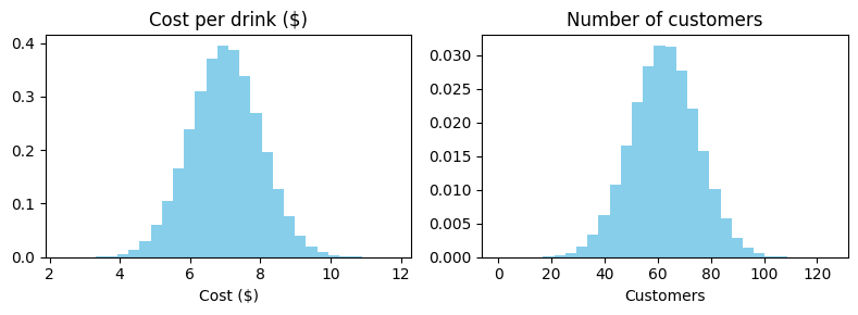
Step 2: Define the possibilities: based on your research, both variables cluster around a typical value with variation tapering off the further you get from it. The cost per drink centers around $7, and the number of customers centers around 60-65 people. This ‘cluster around a middle’ pattern makes the normal (bell-curve) distribution the perfect model for our data.
Step 3: Run the simulations: write your profit function that decides if you are doing this or not and run the simulation 1M times
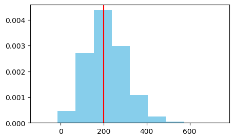
Step 4: Plot the outcomes: now that you have 1M profit values from randomly chosen variables you can plot the outcome to see the range of money you could make
Step 5: Decide feasibility: find the % of your cutoff that decides if this is worth your time (>=$200)
Code
# code-fold: falseimport numpy as npimport pandas as pdimport matplotlib.pyplot as pltsims =1000000selling_price =12cost_price = np.random.normal(7, 1, sims)num_customers = np.random.normal(62.5, 12.5, sims)# First, take a look at the two distributions being combinedfig, axes = plt.subplots(1, 2, figsize=(8,3))axes[0].hist(cost_price, bins=30, density=True, color="skyblue")axes[0].set_title("Cost per drink ($)")axes[0].set_xlabel("Cost ($)")axes[1].hist(num_customers, bins=30, density=True, color="skyblue")axes[1].set_title("Number of customers")axes[1].set_xlabel("Customers")plt.tight_layout()plt.show()total_revenue = num_customers * selling_pricetotal_cost = (num_customers * cost_price) +100profit = total_revenue - total_costplt.figure(figsize = (5,3))plt.hist(profit,density=True, color="skyblue")plt.axvline(200, color ='r')plt.show()print(f"Probability of making at least $200: {100*(profit>=200).sum()/sims:.2f}%")
Probability of making at least $200: 52.93%
Looking at the simulation you see there is a 53% chance you will make at least $200. Maybe it might just be worth the effort after all!
Markov Chain
A Markov chain is a sequence of random variables in which each variable depends only on its immediate predecessor, so the sequence moves at random, each move being determined by its previous position
This chain is often described at “memorylessness” because the probability of the next value depends only on the current value
Sunny or Rainy? A simple weather chain
Let’s better understand this “memorylessness” using a simple weather example. Suppose tomorrow’s weather only depends on today’s weather (not on anything before today):
If it’s Sunny today, there’s an 80% chance it’s Sunny tomorrow and a 20% chance it’s Rainy.
If it’s Rainy today, there’s a 40% chance it’s Sunny tomorrow and a 60% chance it’s Rainy.
We can write this as a transition matrix, where each row is “today” and each column is “tomorrow”:
Notice each row sums to 1, from any given state, we have to end up somewhere tomorrow (possibly the same state).
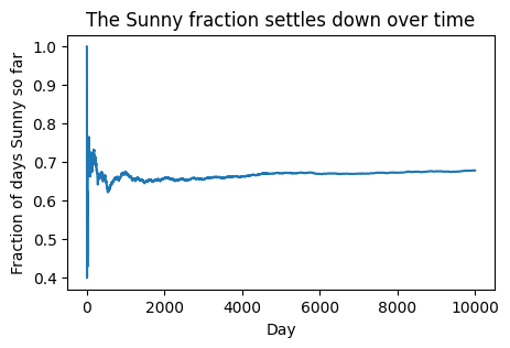
If we start today Sunny and keep hopping from state to state using these probabilities, what fraction of days end up Sunny in the long run? Let’s simulate it and find out.
Tracking the odds, one day at a time
Instead of tracking a single day’s weather, let’s track our belief about the weather as a pair of probabilities. How likely is it to be Sunny, and how likely to be Rainy. Call this the state vector:
Day 4:\[\pi_4 = \pi_3 P = \begin{pmatrix} 0.6752 & 0.3248 \end{pmatrix}\]
Each day the probability of Sunny drops a little: \(1.00 \to 0.80 \to 0.72 \to 0.688 \to 0.675 \to \dots\) but by smaller and smaller amounts. It’s heading somewhere. If we kept going forever, \(\pi_t\) would stop changing entirely.
Let’s see this with code: we’ll simulate one long random walk through this chain (rather than tracking exact probabilities like we just did by hand) and see where it settles.
import numpy as npimport matplotlib.pyplot as pltnp.random.seed(42)# 0 = Sunny, 1 = Rainy. Each row of this matrix is a lookup table:# "given today's weather, what are the odds for tomorrow?"transition_matrix = np.array([ [0.8, 0.2], # today is Sunny -> 80% Sunny tomorrow, 20% Rainy tomorrow [0.4, 0.6], # today is Rainy -> 40% Sunny tomorrow, 60% Rainy tomorrow])days =10000weather =0# day 1 starts off Sunnyhistory = [weather] # keep a record of every day's weatherfor day inrange(days): todays_odds = transition_matrix[weather] # look up today's row weather = np.random.choice([0, 1], p=todays_odds) # randomly pick tomorrow's weather using those odds history.append(weather)history = np.array(history)# Running tally: out of the days seen so far, what fraction were Sunny?sunny_count_so_far = np.cumsum(history ==0)days_so_far = np.arange(1, len(history) +1)running_sunny_fraction = sunny_count_so_far / days_so_farplt.figure(figsize=(5,3))plt.plot(running_sunny_fraction)plt.xlabel("Day")plt.ylabel("Fraction of days Sunny so far")plt.title("The Sunny fraction settles down over time")plt.show()print(f"After {days} days, fraction of days that were Sunny: {running_sunny_fraction[-1]:.2f}")
After 10000 days, fraction of days that were Sunny: 0.68
Conclusion
When we combine the memorylessness of Markov Chains with Monte Carlo simulations we get MCMC simulations. In the previous Markov chain example we saw, no matter which state we’d started in, Sunny or Rainy, the chain eventually “forgets” its starting point and settles into a stationary distribution: about 67% Sunny, 33% Rainy. This is the property MCMC exploits. Instead of designing a chain to describe the weather, we design one whose stationary distribution is the posterior we’re after. Then we just let the chain run and record where it visits. In the next two chapters we’ll see exactly how to build such a chain, first with the Metropolis-Hastings algorithm and then with Gibbs sampling.
Skill Tree Extensions: Recommended Readings
YouTube video on Monte Carlo Simulation by MarbleScience
YouTube video on Monte Carlo Simulation by RiskByNumbers